Basic Setup
%matplotlib inline
import numpy as np
from matplotlib import pyplot as plt
from numpy.random import normal

T = 2.0
n = 100
dt = T / n
First test: solving a simple equation
x = np.zeros(n + 1)

for i in xrange(n):
    x[i + 1] = x[i] + dt + normal(scale = dt)

t = np.linspace(0, T, n + 1)

plt.plot(t, x, '*')
[<matplotlib.lines.Line2D at 0x3a55b10>]
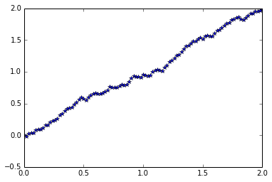
Stochastic maltus model
Problem parameters
r = 1
c = 1
x0 = 1

t = np.linspace(0, T, n + 1)
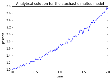
Analytic solution
factor = r - c**2 / 2.0

x = np.ones(n + 1)
w = normal(scale=dt, size=n + 1)
w[0] = 0

x = x0 * np.exp(factor * t + c * w)

plt.plot(t, x)
plt.title('Analytical solution for the stochastic maltus model')
plt.xlabel('time')
plt.ylabel('position')
<matplotlib.text.Text at 0x48dd910>
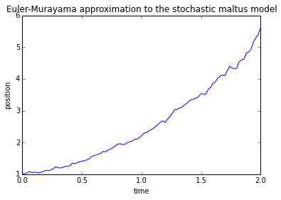
Euler-Murayama approximation
x2 = np.zeros(n + 1)
x2[0] = x0

for i in xrange(n):
    xi = x2[i]
    x2[i + 1] = xi + r * xi * dt + c * xi *  normal(scale = dt)

plt.plot(t, x2)
plt.title('Euler-Murayama approximation to the stochastic maltus model')
plt.xlabel('time')
plt.ylabel('position')
<matplotlib.text.Text at 0x4dd5b50>
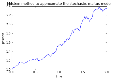
Milstein method
x3 = np.zeros(n + 1)
x3[0] = x0

for i in xrange(n):
    xi = x3[i]
    wi = normal(scale = dt)
    x3[i + 1] = xi + r * xi * dt + c * xi *  wi + 0.5 * c * xi * c * (wi**2 - dt)

plt.plot(t, x3)
plt.title('Milstein method to approximate the stochastic maltus model')
plt.xlabel('time')
plt.ylabel('position')
<matplotlib.text.Text at 0x4dcc590>
Qualitative comparison
plt.plot(t, x, t, x2, t, x3)
plt.title('Qualitative comparison of the three methods')
plt.xlabel('time')
plt.ylabel('position')
plt.legend(('Analytic', 'Euler-Murayama', 'Milstein'), loc='upper left')
plt.grid()
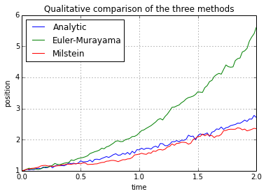
As it was expected, euler’s method is more prone to error than Milstein’s correction. It remains to make a comparison of results for different values of the parameters. It is not expected any important difference in the results if varying initial conditions
Appendix: Routines for solving sde
It is straightforward to write routines for solving stochastic equations with Euler-Murayama’s and Milstein’s methods. For later, convenience, they are written here.
def emurayama(T, timesteps, x0, alpha, beta):
    '''
    x = emurayama(T, timesteps, x0, alpha, beta)

    solves the stochastic differential equation

    dx = alpha * dt + beta * dw
    x(0) = x0

    with Euler-Murayama method.

    input:

              T = Final time.
      timesteps = Number of timesteps to use.
             x0 = initial condition.
    alpha, beta = equation parameters. Must be functions like this:

    x = alpha(xi, ti),

    i.e. its input must be two floating point numbers and must return another floating point.
    (No vectorization, due to the recursive definition of the algorithm)

    returns:

        array of lenght timesteps + 1 with the result.
    '''

    x = np.zeros(timesteps + 1)
    x[0] = x0
    ti = 0.0
    dt = float(T) / timesteps

    for i in xrange(timesteps):
        xi = x[i]
        ti += dt
        x[i + 1] = xi + alpha(xi, ti) * dt + beta(xi, ti) *  normal(scale = dt)

    return x

def milstein(T, timesteps, x0, alpha, beta, diff_beta):
    '''
    x = milstein(T, timesteps, x0, alpha, beta)

    solves the stochastic differential equation

    dx = alpha * dt + beta * dw
    x(0) = x0

    with Milstein's method.

    input:

              T = Final time.
      timesteps = Number of timesteps to use.
             x0 = initial condition.
    alpha, beta = equation parameters. Must be functions like this:

    x = alpha(xi, ti),

    i.e. its input must be two floating point numbers and must return another floating point.
    (No vectorization, due to the recursive definition of the algorithm)

    diff_beta = partial derivative of beta, respect to x.

    returns:

        array of lenght timesteps + 1 with the result.
    '''

    x = np.zeros(timesteps + 1)
    x[0] = x0
    ti = 0.0
    dt = float(T) / timesteps

    for i in xrange(timesteps):
        xi = x[i]
        ti += dt
        wi = normal(scale = dt)
        x[i + 1] = xi + alpha(xi, ti) * dt + beta(xi, ti) *  wi + 0.5 * beta(xi, ti) * diff_beta(xi, ti) * (wi**2 - dt)

    return x